Background and motivation
The monitoring problem
- Runtime monitoring checks a system's actual behaviour against a formal specification.
- Online monitoring is done while the system is running.
- Offline monitoring is done on a log after the system has completed.
We focus on the online monitoring problem.
MonPoly
MonPoly is a runtime monitor. Its policies are written in metric first-order temporal logic (MFOTL), which adds temporal operators to first-order logic. Each operator carries an interval I that restricts the time points relevant to it.
| Next | ∘Iφ | Always | □Iφ |
| Previous | ∙Iφ | Historically | ■Iφ |
| Until | φUIψ | Eventually | ◊Iφ |
| Since | φSIψ | Once | ⧫Iφ |
The temporal operators are on the left, the syntactic sugar built from them on the right.
- Time point: a time-stamped collection of events (predicates), often referred to by an integer index.
- Time stamp: a moment in time, e.g. seconds since the Unix epoch.
The thesis defines the logic in §2.1 Metric First-Order Temporal and Dynamic Logic and introduces the tool in §2.2 MonPoly.
Time-series databases
A time-series database is optimized for inserting and retrieving temporal data. We use QuestDB:
- It is largely compatible with PostgreSQL.
- It adds a
TIMESTAMPdata type to the usual typesINT,STRING, etc. - Each table has a dedicated time stamp column, analogous to an index column.
More in §2.3.1 QuestDB.
Monitor vs. database
| Monitor (MonPoly) | Time-series database (QuestDB) | |
|---|---|---|
| Good when | data changes often the policy changes rarely | data stays almost constant queries vary and are frequent |
| Bad when | the policy changes frequently | data changes rapidly |
Combining monitoring and a time-series database
We build a wrapper that logs and monitors the same data. It:
- provides the functionality of both a monitor and a time-series database,
- allows us to offer a policy change method,
- gives MonPoly a more accessible interface, for web services and distributed systems,
- increases fault tolerance.
From signature to database schema
Each predicate of a MonPoly signature becomes a table, with one column per
attribute plus the time point tp and the time stamp ts. One
more table records every time point, including those without events.
CREATE TABLE P(x1 INT, x2 STRING,
               tp INT,
               ts TIMESTAMP)
               timestamp(ts);
CREATE TABLE Q(x1 INT, x2 INT,
               tp INT,
               ts TIMESTAMP)
               timestamp(ts);
CREATE TABLE R(x1 INT, x2 STRING,
               x3 STRING,
               tp INT,
               ts TIMESTAMP)
               timestamp(ts);
CREATE TABLE time_points
               (tp INT,
               ts TIMESTAMP)
timestamp(ts);P(id:int, act:string)
Q(id1:int, id2:int)
R(int, string, string)The thesis explains the mapping in §2.3.2 Time Series Databases for Runtime Monitoring.
Agenda
- The wrapper: its REST API, architecture and data flow.
- Algorithm and policy change: relative intervals and their extension.
- Partial policy change: work in progress inside MonPoly.
- Evaluation and outlook.
The wrapper
The REST API
| Monitor and log | QuestDB connection |
|---|---|
/ (info page) | /db-set-user |
/set-policy | /db-set-password |
/set-signature | /db-set-host |
/start-monitor | /db-set-pgsql-port |
/stop-monitor | /db-set-influxdb-port |
/change-policy | /db-set-database |
/get-policy | /db-get-user |
/get-signature | /db-get-password |
/reset-everything | /db-get-host |
/log-events | /db-get-pgsql-port |
/get-events | /db-get-influxdb-port |
/get-most-recent | /db-get-database |
Every endpoint is described, with example calls, in §3.2 The REST API.
Architecture
Data flow
The wrapper checks incoming events before they reach MonPoly, and faulty input is reported instead of stopping the monitor: fault tolerance increases compared to MonPoly alone.
Algorithm and policy change
Policy change
- A policy change starts a new monitor with the new policy.
- Goal: the new monitor evaluates the new policy at the current time point just as if it had seen the same trace as the old monitor.
- Naive approach: read the entire trace again.
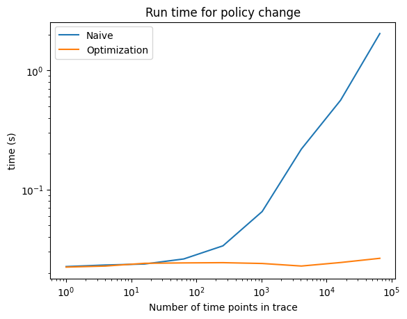
- Idea: reduce the trace by removing events that do not influence how the new policy is evaluated.
Optimization example
φ=(P(x,“a”)S[0,30)Q(x,2))∧(¬R(y,“c”,z)S[20,60)P(y,z))- Relative interval: RI(φ)=(−60,0]
- Extended relative intervals: ERI(φ)=amp;P(∗,∗)amp;P(∗,“a”)amp;Q(∗,2)amp;R(∗,“c”,∗)amp;amp;amp;amp;amp;→(−60,−20]amp;→(−30,0]amp;→(−30,0]amp;→(−60,0]
Time points whose time stamps lie outside {current time stamp}⊕RI(φ) do not change the evaluation of φ at the current time point.
Interval operators
Let I and J be two intervals. Then
- I⊕J={i+j∣i∈I,j∈J}, for example [0,3]⊕[−2,4]=[−2,7];
- I⋓J is the smallest interval that contains every element of I or J, for example [−4,1]⋓[4,5]=[−4,5].
Relative intervals
The relative interval of a formula φ, RI(φ)⊆Z, is defined inductively over the formula structure [3]:
Definition 4.1 in the thesis also covers the MFODL operators.
Extended relative intervals: operators
A map from masked predicates to intervals replaces the single interval, so new operators are needed. Let M and N be two masked predicate maps and T an interval:
M⋓¨N=T⋓˙M=T⊕˙M=amp;{p(l)→(I⋓J)∣p(l)→I∈M and p(l)→J∈N}amp;∪{p(l)→I∣p(l)→I∈M and p(l)∈keys(M)∖keys(N)}amp;∪{p(l)→I∣p(l)→I∈N and p(l)∈keys(N)∖keys(M)}amp;{p(l)→(T⋓I)∣p(l)→I∈M}amp;{p(l)→(T⊕I)∣p(l)→I∈M}Extended relative intervals
The definition follows that of relative intervals; what changes is marked.
We proved that this definition is a correct approximation: it extracts all time points from a trace that are needed, and φ evaluates the same on the original trace and on the extraction.
Definition 4.11; the proof is in §4.3.1 Correctness.
Extended relative intervals in the example
φ=(P(x,“a”)S[0,30)Q(x,2))∧(¬R(y,“c”,z)S[20,60)P(y,z))- Relative interval: RI(φ)=\blu(−60,0]
- Extended relative intervals: ERI(φ)=amp;P(∗,∗)amp;P(∗,\acc“a”)amp;Q(∗,\acc2)amp;R(∗,\acc“c”,∗)amp;amp;amp;amp;amp;→\acc(−60,−20]amp;→\acc(−30,0]amp;→\acc(−30,0]amp;→\acc(−60,0]
What the query keeps
On a random trace, each masked predicate keeps only the events in its own interval. Everything else in (−60,0] is skipped, although the plain relative interval would read it. An event appears in every row whose mask it matches.
The thesis shows the same picture next to §4.3 Relative Interval Extension.
From extended relative intervals to SQL
Each masked predicate becomes a condition on its table; the time points table is queried with the relative interval of the whole formula.
SELECT * FROM P WHERE
    (time_stamp > <NOW>-60 AND time_stamp <= <NOW>-20)
    OR
    (x2 = "a" AND
    time_stamp > <NOW>-30 AND time_stamp <= <NOW>-0);
SELECT * FROM Q WHERE
    (x2 = 2 AND
    time_stamp > <NOW>-30 AND time_stamp <= <NOW>-0);
SELECT * FROM R WHERE
    (x2 = "c" AND
    time_stamp > <NOW>-60 AND time_stamp <= <NOW>-0);
SELECT * FROM time_points WHERE
(time_stamp > <NOW>-60 AND time_stamp <= <NOW>-0);Converting the database result
QuestDB's answer is turned into the wrapper's JSON log format, and from there into a MonPoly log that the new monitor reads before it switches to standard input.
[{"R":[]},
 {"Q":[[0,8,65536,"Thu, 01 Jan 1970 00:00:01 GMT"]]},
 {"P":[]},
 {"time_points":[[65536,"Thu, 01 Jan 1970 00:00:01 GMT"],
[65537,"Thu, 01 Jan 1970 00:00:02 GMT"]]}][{"predicates":[{"name":"Q","occurrences":[[0,8]]}],
"timepoint":65536,"timestamp":"1970-01-01 00:00:01"},
{"predicates":[],
"timepoint":65537,"timestamp":"1970-01-01 00:00:02"}]@1 Q(0,8);
@2 ;Partial policy change (work in progress)
Partial policy change in MonPoly
- Only for first-order logic operators above temporal operators.
- Named formulas:
NAME[f1, name1] OR NAME[f2 AND f3, name2] - We added data types for
NAMEto MonPoly and updated the formula parser forNAMEconstructs. - We started work on commands that add or remove conjuncts and disjuncts:
>remove_part <name><
>add_conjunct <name1> <name2> <formula><
>add_disjunct <name1> <name2> <formula><Partial policy change: example
φ=(P(x,“a”)S[0,30)Q(x,2))∧(¬R(y,“c”,z)S[20,60)P(y,z))With names for its parts, the policy becomes
NAME[(P(x,"a") SINCE[0,30) Q(x,2)), part1] AND
NAME[(NOT (R(y,"c",z)) SINCE[20,60) P(y,z)), part2]>add_disjunct part1 part3 'NOT P(2,"b")'<(NAME[P(x,"a") SINCE[0,30) Q(x,2), part1] OR
NAME[NOT P(2,"b"), part3]) AND
NAME[NOT (R(y,"c",z)) SINCE[20,60) P(y,z), part2]Partial policy change: next steps
- Compute the internal state for formula parts that are added.
- Combine the existing state with the state of the new formula.
- Update the state when a formula part is removed.
Evaluation
Overhead of the wrapper
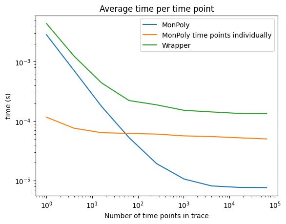
- A random policy with intervals bounded by [0,20).
- A random trace with 4i time points, for i=0,…,8.
- We measure the time MonPoly takes to monitor these traces;
- the time MonPoly takes when the time points are sent individually instead of in one file, which better simulates online monitoring;
- and the time the wrapper takes to monitor the traces.
- This was done 100 times, with 100 different policies.
The thesis reports this experiment in §5.4.1 Wrapper vs. MonPoly.
Overhead of the wrapper: results
Overhead of the wrapper: conclusion
More detailed profiling is required. Possible sources of the overhead:
- converting our JSON log format to the MonPoly format;
- the wrapper sends time points to MonPoly synchronously;
- the wrapper goes over the events once to send them to MonPoly and again later to send them to QuestDB.
Policy change optimization
- A policy change between 2 randomly generated formulas.
- Intervals in the policies are bounded by [0,20).
- Random traces with 4i time points, for i=0,…,8.
- Load the trace into the wrapper, then start the policy change.
- This was done 100 times, for 100 different policy pairs.
Policy change optimization: results
Outlook
Outlook
- Reduce the overhead of the wrapper: profile it in more depth, and send time points asynchronously, without waiting for a response before sending the next one.
- Speed up the policy change: check constraints on variables in formulas, such as x<20, more thoroughly.
- Continue the partial policy change within MonPoly.
The thesis closes with §6 Conclusion.